Skewness and Kurtosis
Skewness is a measure of the asymmetry or symmetry of a a data distribution.
A distribution , or data set, is symmetric if it looks the same to the left and right of the center point.
No skewness=symmetric curve
Types of skewness
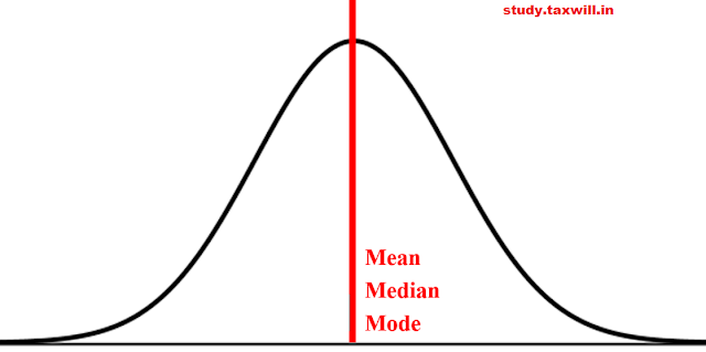
1)No skewness(Zero skewness): if the values of variable are equidistance from the mean have equal frequency ,then the distribution is said to have symmetric or zero skewness. Normal distribution visual, also known as a bell curve. It is a symmetrical graph with all measures of central tendency in the middle
Mean=median=mode
2)Positive skewness right skewed: If the frequency of the values of the variable lower than the mean have high frequencies compared to the frequencies associated with the values of variables higher than the mean.
mean>median >mode
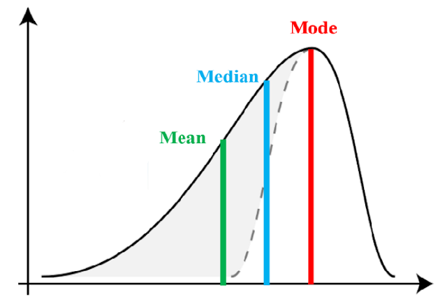
3)Negative skewness left skewed:
mode>median>mean
For the left graph since the tail is to the left, it is left-skewed (negatively skewed) and the right graph has the tail to the right, so it is right-skewed (positively skewed).
How about deriving a measure that captures the horizontal distance between the Mode and the Mean of the distribution? It’s intuitive to think that the higher the skewness, the more apart these measures will be.
So let’s jump to the formula for skewness now
Division by Standard Deviation enables the relative comparison among distributions on the same standard scale. Since mode calculation as a central tendency for small data sets is not recommended, so to arrive at a more robust formula for skewness we will replace mode with the derived calculation from the median and the mean.
Replacing the value of mode in the formula of skewness, we get:
Kurtosis
What is Kurtosis and how do we capture it?
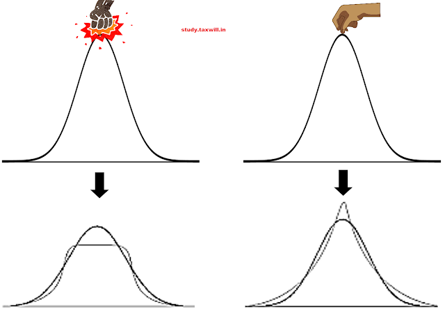
Think of punching or pulling the normal distribution curve from the top, what impact will it have on the shape of the distribution? Let’s visualize:
kurtosis is a a measure of whether the data are heavy -tailed or light -tailed relative to a normal distribution.
So there are two things to notice — The peak of the curve and the tails of the curve, Kurtosis measure is responsible for capturing this phenomenon. The formula for kurtosis calculation is complex (4th moment in the moment-based calculation) so we will stick to the concept and its visual clarity. A normal distribution has a kurtosis of 3 and is called mesokurtic. Distributions greater than 3 are called leptokurtic and less than 3 are called platykurtic. So the greater the value more the peakedness. Kurtosis ranges from 1 to infinity. As the kurtosis measure for a normal distribution is 3, we can calculate excess kurtosis by keeping reference zero for normal distribution.
Now excess kurtosis will vary from -2 to infinity.
Excess kurtosis=kurtosis-3
Excess Kurtosis for Normal Distribution = 3–3 = 0
The lowest value of Excess Kurtosis is when Kurtosis is 1 = 1–3
= -2
So we can conclude from the above discussions that the horizontal push or pull distortion of a normal distribution curve gets captured by the Skewness measure and the vertical push or pull distortion gets captured by the Kurtosis measure. Also, it is the impact of outliers that dominate the kurtosis effect which has its roots of proof sitting in the fourth-order moment-based formula. I hope this blog helped you clarify the idea of Skewness & Kurtosis in a simplified manner, watch out for more similar blogs in the future.
FOLLOW US ON YOUTUBE
https://www.youtube.com/channel/UC3jRTLRqVxbB0KjPM65aMtA


Kurtosis does not refer to vertical height, peakedness, flatness, or "push and pull." You can have infinitely peaked distributions with very low kurtosis, and you can have low, perfectly flat-topped distributions with very high kurtosis. Examples are given on the current Wikipedia page.
ReplyDelete